First Layer Error Detection Report
Andrew Viola, Maxwell KawadaFall 2024 ECE 4554/5554 Computer Vision: Course Project
Virginia Tech
GitHub Repository
Visit here for the project proposal
Abstract
First-layer adhesion error is a common issue encountered by novices during 3D printing, resulting in print defects and failed prints. Stemming from improperly set z-offset, an inconsistent bed mesh, or a sagging gantry, these issues prevent the first layer of the print from setting in the correct position causing time and filament to be wasted if left unnoticed.In a series of two steps, we used computer vision from a camera mounted above a 3D printer bed to analyze the quality of the first layer to ensure that the rest of the print would be successful. First, a trained YOLO model is used to detect the “spaghetti-ing” of the filament, followed by a script to ensure the first layer is in the correct position while identifying the quality from the shape of the printing patterns.
With this system, we were able to identify print failures that occurred via spaghetti-ing, sending a call to the printer to stop the printing process. We were also able to correctly identify when and how many parts of an attempted print were missing, along with the reasons behind low-quality yet functional prints.
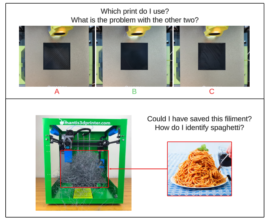
Teaser
Introduction
As 3D printing technology becomes more affordable, it is increasingly more accessible to a broader range of consumers. However, with the greater install base of 3D printers, common challenges faced by experienced hobbyists are encountered by new users who may not know how to solve them. One such issue is often first-layer adhesion.First-layer adhesion can arise from an improperly set z-offset, an inconsistent bed mesh, or a sagging gantry. These varying issues can all lead to significant print defects. One such defect is the object coming loose from the bed mid-print, causing a print failure. Another example of a defect is elephant foot, where the bottom layer spreads beyond the intended dimensions, causing accuracy issues. A proper first layer is the first step in achieving successful prints.
Companies such as Bambu Lab and Creality utilize micro LiDAR sensors, which can measure depth in micrometers. They utilize this technology to scan the first layer and measure any inconsistencies with the height of the layer. Combining this with a proprietary machine learning algorithm, they can detect any irregularities within the height and pause the print. While this method is consistent and can work well, it is proprietary to Bambu Lab and Creality. Its implementation is also different between the two companies, along with no broader support for other printers, such as a DIY printer. In addition to this, it requires extra hardware on the tool head, increasing costs and weight.
Taking an existing camera found on many consumer and DIY printers, adding extra cost and weight can be avoided. It also lets any user be able to take advantage of the first layer detection without having to enter a proprietary ecosystem. By utilizing computer vision, it is possible to ensure an optimal first layer, reducing the risk of common print defects and improving the overall print quality of the object being printed.
Approach
To perform a computer vision project, we must first set up a camera to obtain information from. By modding a Voron Switchwire, a popular DIY 3D printer, a camera mount can be printed and attached to the top to obtain a birds-eye view of the print bed. To ensure that sufficient lighting was supplied for the camera, a lamp was placed above the camera to shine on the print bed. Utilizing this setup, we were able to obtain quality camera footage of the print bed as the 3D printer is actively printing. This camera provides a live feed synchronized to the printer. This provides a live view to the user along with API access to grab the current frame at a moment’s notice. Most DIY printers utilize Moonraker as the backend to their frontend. Moonraker exposes various systems to the user in the form of an API. One such system is the camera connected to the printer. Utilizing Moonraker’s API access [1], a picture of the bed is taken after the entire first layer has been completed, along with pictures being taken periodically to inspect the current layer.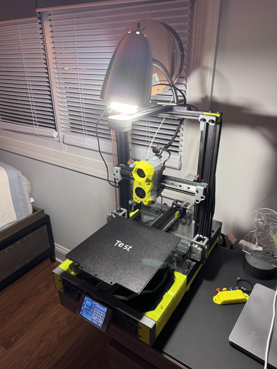
Figure 1: The test setup
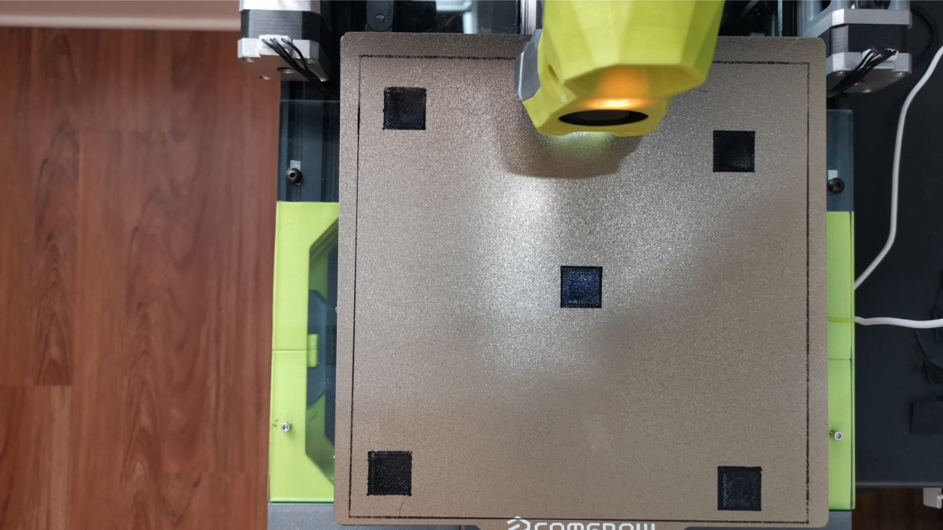
Figure 2: Output of the camera
The code is split into three main phases, with each phase corresponding to a specific detection being done. However, prior to any detection being done, a skew correction needs to occur. As seen from the figure above, the build plate is slightly rotated clockwise, along with having extra information on the sides of the plate. To account for this, a perspective transformation is done on the image. The goal is to have the output frame be a perfect bird’s eye view. Due to the nature of planar 3D printing, layers of a print are calculated and can be viewed as a simulated perfect layer from the top-down perspective. This can be viewed in Figure 3. Utilizing this perfect simulated view, the corners are manually measured in the simulated view and the camera view. Then the homography matrix is solved for and applied to the camera view in order to create an accurate bird’s eye view representation of the camera view. This ensures that the camera view is in the same orientation, scale, and perspective as the simulation. This can be seen in Figure 4. Overlaying the two images shows that the corrected camera view matches the perfect simulated layer. This can be seen in Figure 5. With the newly corrected view, the first phase of detection can occur.
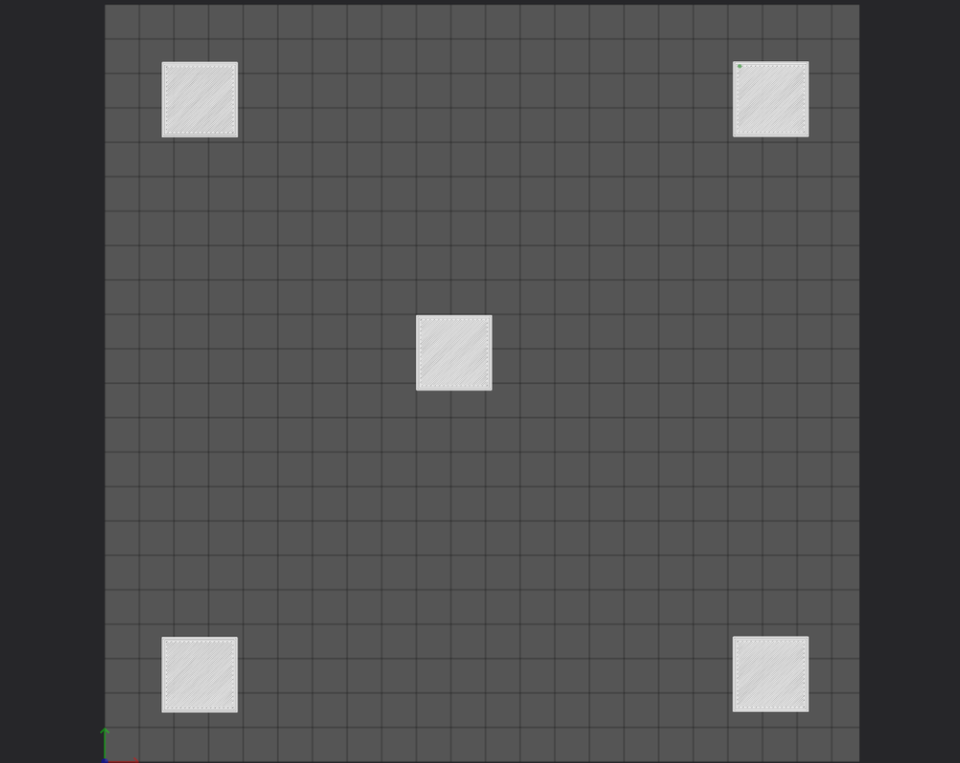
Figure 3: Simulated First Layer
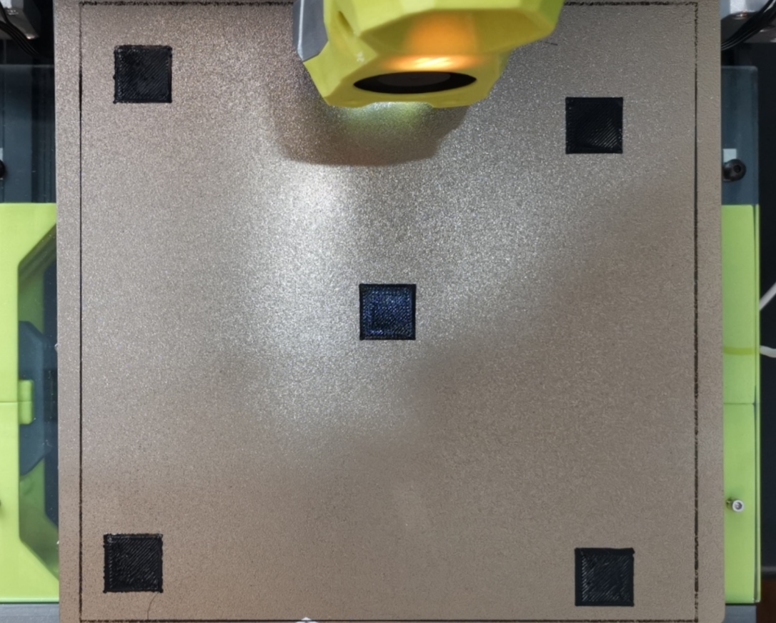
Figure 4: Skew Corrected Camera View
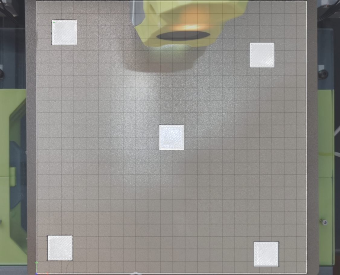
Figure 5: Simulated and skew corrected view overlaid
The first detection is a missing object detection. This is done by comparing the expected perfect first layer and the actual correct camera view. The camera view is masked to show only the first layer. Then thresholding is applied so the areas missing become 255 and the layers become 0. This highlights the extreme difference between the perfect layer and a layer of missing objects. Afterward, a percent difference calculation is done to compare how different the perfect layer is from the camera view layer. Above a 25% difference or a 0% difference deems that there are most likely missing objects. The reasoning for a 0% difference resulting in missing objects is that if every object is missing on the layer, then the thresholding would result in a binarized output that looks identical to the mask.
The second detection is determining if the z-offset is too low, too high, or just perfect. We do this by again taking the corrected camera view and the perfect view and masking out the camera view to be only the layer. We then take the gradient in the X and Y directions and aggregate them to obtain the magnitude of each pixel.
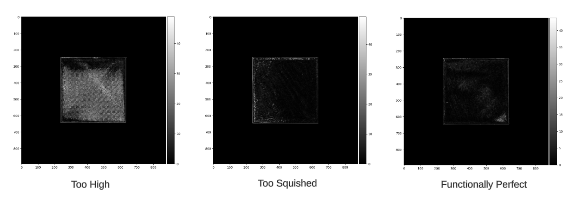
Figure 6: Gradient Analysis
Then we calculate the mean gradient and the variance of the gradient. In addition to this, we use canny edge detection to get the edge density of the masked camera view. Utilizing carefully adjusted thresholds (found through experimental methods) of these three values, we can determine if the layer’s height is too squished, too tall, or just perfect. We often refer to low z-offset prints as being “squished” due to the filament being crammed together after being placed onto the print bed. With high z-offset prints, we often see the opposite, and instead, gaps will appear on the surface and edges of the print. Tall first layers often have attributes such as more defined edges and a higher variance. While squished layers often have less defined edges and a low variance. Perfect first layers meet somewhere in the middle (of course, this is very generally speaking, outliers can occur). The thresholds selected earlier correspond to the boundaries of what we deem an acceptable distribution of filament onto the print bed, so between the thresholds is our functional range, and everything outside those thresholds is considered poor quality.
The last detection is stray filament detection, better known as spaghetti detection. This is when an excess amount of filament is being printed and not sticking to the intended point. Beyond the first layer printed, every 30 seconds, a frame of the camera is taken and fed into a YOLO11 model. The YOLO11 mode is trained to identify images of 3D printer spaghetti-ing. YOLO, standing for “You Only Look Once,” is an object detection algorithm made by Joseph Redmon and Ali Farhadi that works in real time, utilizing a convolutional neural network [1]. YOLO11, produced by Ultralytics, provides an upgraded and lightweight framework for the famous YOLO computer vision model that we used to train and perform inference[2]. Then, by using a roboflow dataset made by the user “3D Printing Failure” that contains both training and testing data of 3D printer spaghetti, we were able to easily train the YOLO11 model which would now detect when a print begins to fail [3]. If the print fails and the YOLO model detects the spaghetti, a simple pause command is sent to the printer, which saves time and filament for the users. This continues until the end of the print occurs.
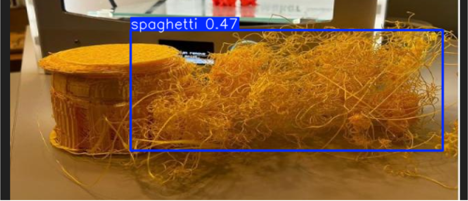
Figure 7: Output of the YOLO model
If the print completes all phases of our code, then we have deemed the first layer of the print to be up to our quality standard. The 3D printer will then continue its printing operations on a well-structured first layer, and the user will save plenty of time and money by avoiding defective prints and saving filament.
Experiments and Results
As previously mentioned, a camera and lamp attached to the Voron Switchwire were used as the experimental setup. Python was used with OpenCV, Numpy, and Requests libraries in order to interact with the 3D printer.To test skew correction, Python was used to grab the current frame and the current layer of the 3D print. Naively assuming that the build plate was the exact size as the build volume, the four corners of the build plate were used as reference points for a 2D projective transformation. When applying the homography matrix to the camera view, the orientation and perspective seemed to be solved, however, the scale was off. This can be seen in the figure below.
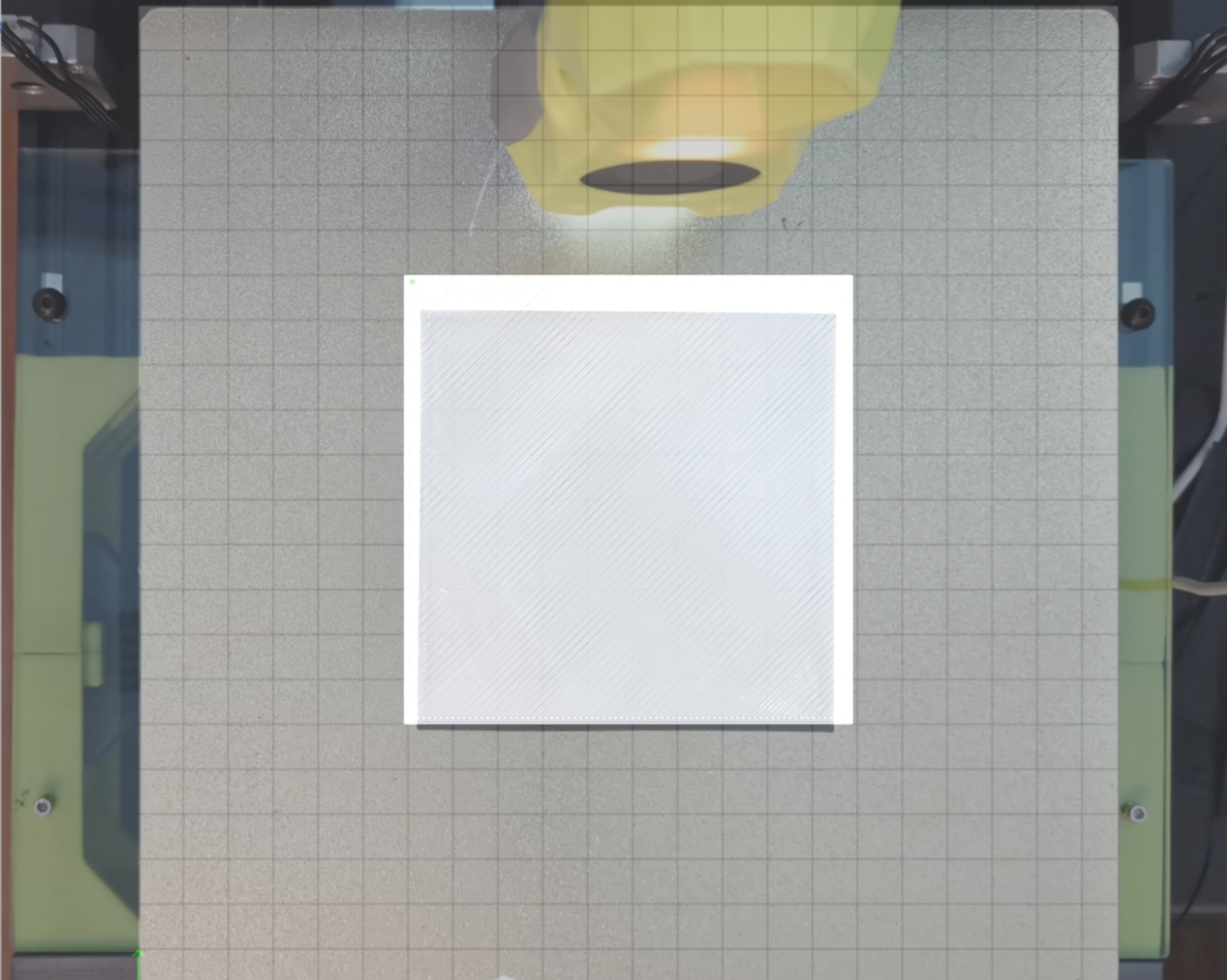
Figure 8: After skew correction, scale is off
After realizing that the build plate was larger than the build volume, a rectangle was printed around the build volume to discover the bounds of the print volume. This can be seen in the figure below.
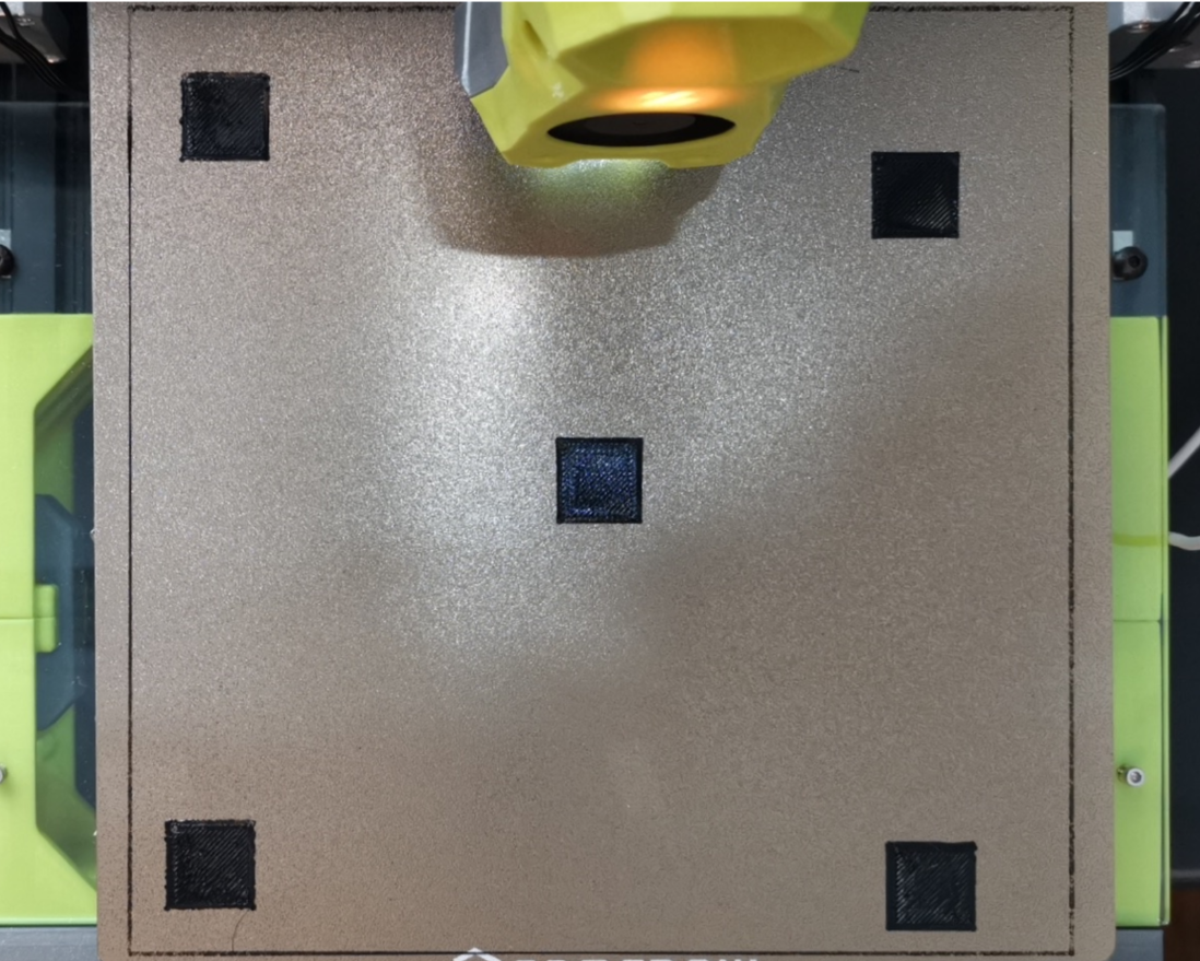
Figure 9: Printed rectangle around the build volume
Measuring out the new corners and applying the new homography matrix demonstrates that the correction seems to be applied correctly. See Figures 3-5 for an example of a correctly applied transformation. Furthermore, the correction was tested on thirty different first layers, and the average similarity between the corrected camera and the perfect layer was 99.02%. The average similarity was calculated by masking out the general area of where the objects should be, and then doing a binary threshold, revealing where the real-world object is. Then doing an SSIM (structural similarity index measurement) calculation with the thresholded image and the expected output reveals the similarity [4]. A table with all of the results can be found below.
| File | Similarity |
|---|---|
| functionallyPerfect.png | 99.57% |
| perfectVoron.png | 98.67% |
| perfectBoat.png | 99.57% |
| perfectHotend.png | 98.93% |
| perfectTest.png | 99.21% |
| functionalExtruder.png | 99.00% |
| perfectFox.png | 98.89% |
| perfectFlower.png | 98.74% |
| perfectWatch.png | 99.32% |
| tooSquished.png | 99.57% |
| squishedVoron.png | 98.67% |
| squishedBoat.png | 99.57% |
| squishedHotend.png | 98.93% |
| squishedTest.png | 99.21% |
| squishedExtruder.png | 99.00% |
| squishedFox.png | 98.89% |
| squishedFlower.png | 98.74% |
| squishedWatch.png | 99.32% |
| squishedPrusa.png | 97.88% |
| highBoat.png | 99.57% |
| tooHigh.png | 99.57% |
| highVoron.png | 98.67% |
| highHotend.png | 98.93% |
| highTest.png | 99.21% |
| highExtruder.png | 99.00% |
| highFox.png | 98.89% |
| highFlower.png | 98.74% |
| highWatch.png | 99.32% |
| highPrusa.png | 97.88% |
| Average | 99.02% |
Table 1: Accuracy of prospective transformation with respect to simulated layer
Missing object detection experimentation was a bit more difficult. Initially set thresholds were used to determine the missing threshold. However, due to lighting conditions, parts of the first layer would appear as if it was missing. This can be seen in the figures below.
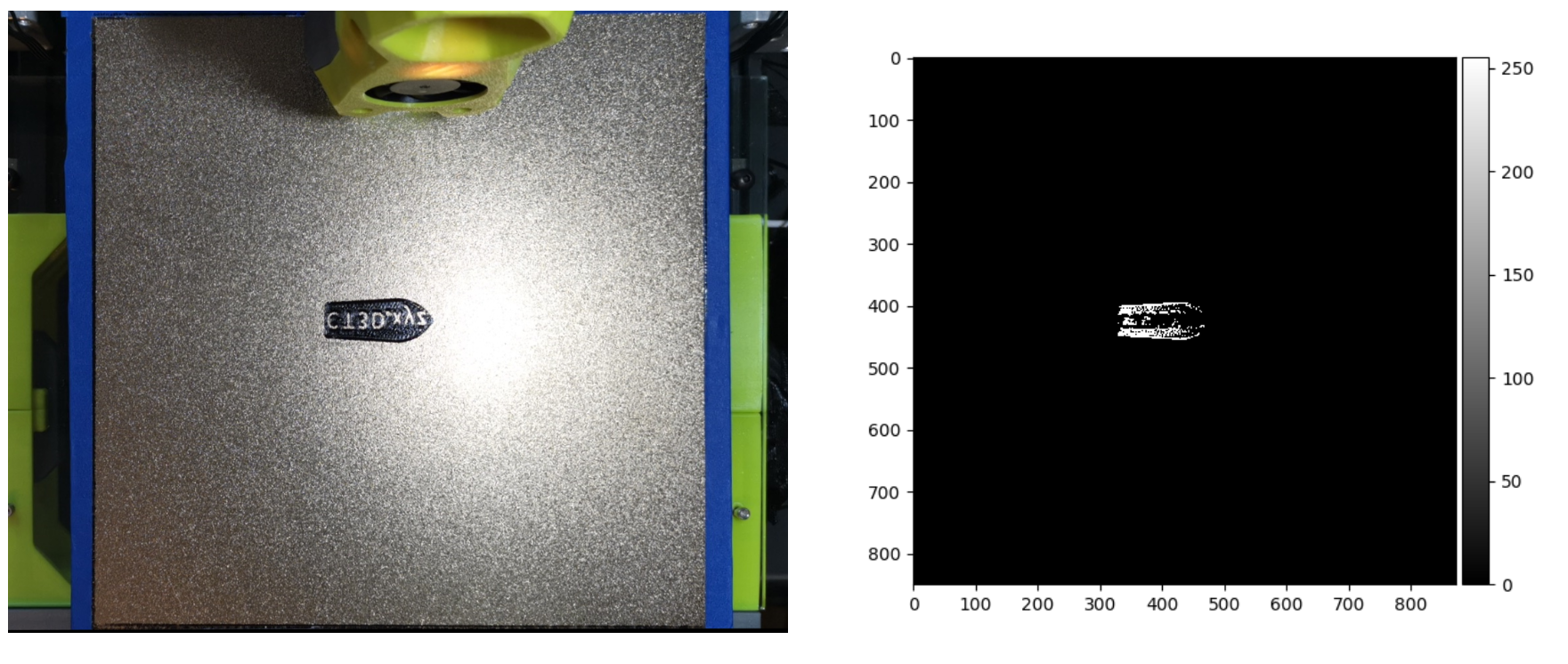
Figure 10: Image on the left is the original image, the right is the binarized view after thresholding. White indicates existing objects
To accommodate for this, a scaled dynamic threshold was implemented. This takes the max intensity value in the layer and uses 4/10th of that value as the threshold. This worked a bit better with the samples showing up mostly correct. The new threshold examples can be seen below.
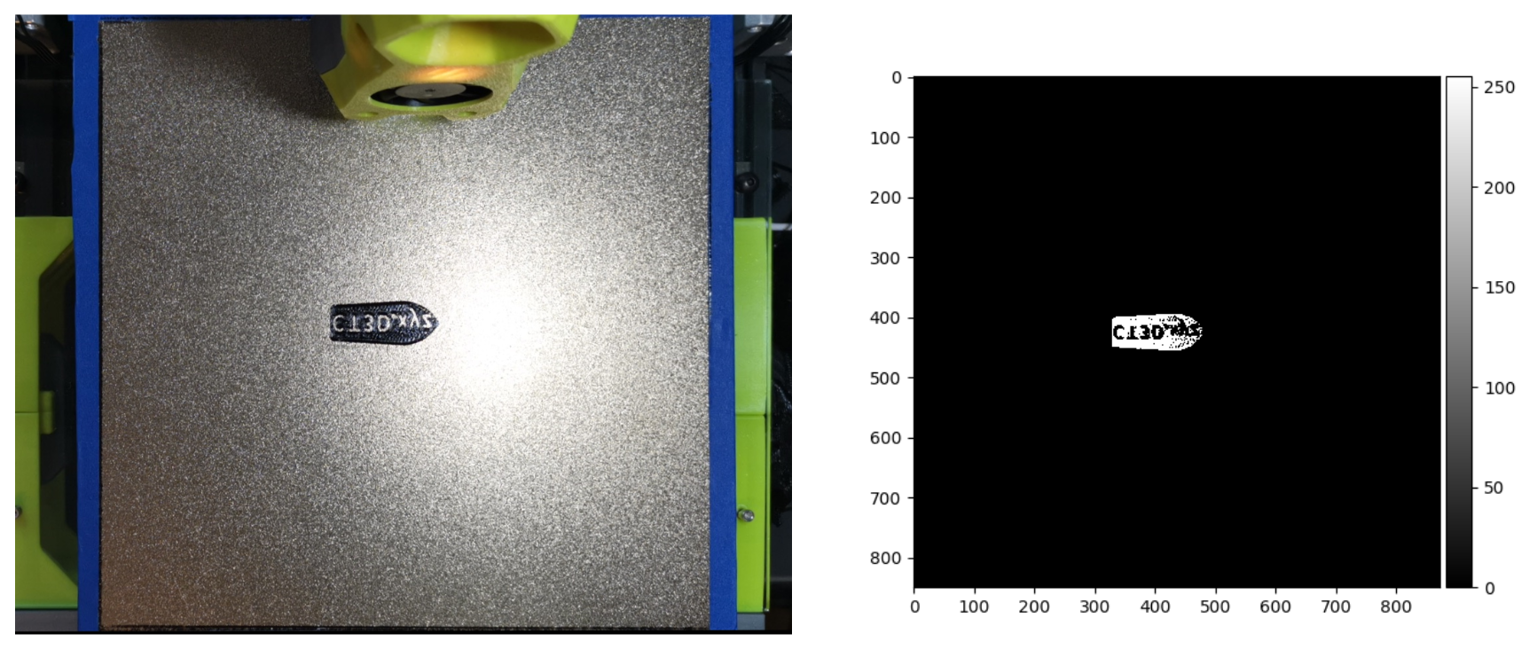
Figure 11: Improved thresholding
With improved thresholding, the first layers of 10 varying objects were used to test if our code can recognize if the layer has been completed. For the set of 10 first-layer images, 5 of these images had a complete layer with all objects of the layer present, whereas the remaining first-layer images had missing objects or were completely absent. Two of the missing object images were photoshopped to remove parts of the first layer, while in the other three missing object images, the objects were physically removed. Below is a table of the results, indicating the percent difference between objects and whether the program identified missing objects appropriately.
| File | Percent Difference | Expected | Output |
|---|---|---|---|
| missingFox.png | 9.25586 | Missing | Normal |
| missingPS5.png | 50.03465 | Missing | Missing |
| missingBenchy.png | 99.55685 | Missing | Missing |
| missingFlower.png* | 27.35719 | Missing | Missing |
| missingVoron.png* | 57.84845 | Missing | Missing |
| perfectTest.png | 3.85948 | Normal | Normal |
| workingPS5.png | 3.09121 | Normal | Normal |
| workingBenchy.png | 23.97175 | Normal | Normal |
| perfectPrusa.png | 0.77499 | Normal | Normal |
| perfectVoron.png | 5.18713 | Normal | Normal |
Table 2: Object Detection Test Results. 90% of the tests resulted in the correct class
Note: The * indicates an image that was digitally altered to remove part of the layer.
missingFox.png resulted in an incorrect prediction of normal due to its low percent error.
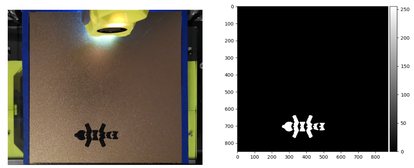
Figure 12: missingFox.png
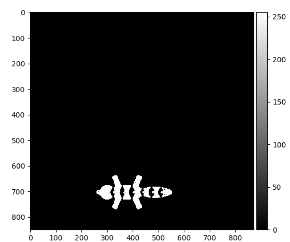
Figure 13: missingFox.png's simulated layer after binarized thresholding
Looking at Figures 12 and 13, they demonstrate that the machine correctly identified the layer, but when comparing it to the proper first layer, the missing part is very small. This leads to a small percent difference calculation and thus an incorrect identification.
Determining whether the first layer was at the proper height was the most challenging by far. Depending on how squished an object is can determine the variance of the gradients along with more defined edges. This is because rather than having a surface that appears extremely flat (meaning no variance), it can create ridges in the first layer, highlighting new edges. Below is an example of layers that are all too squished, but have different-looking gradient plots.
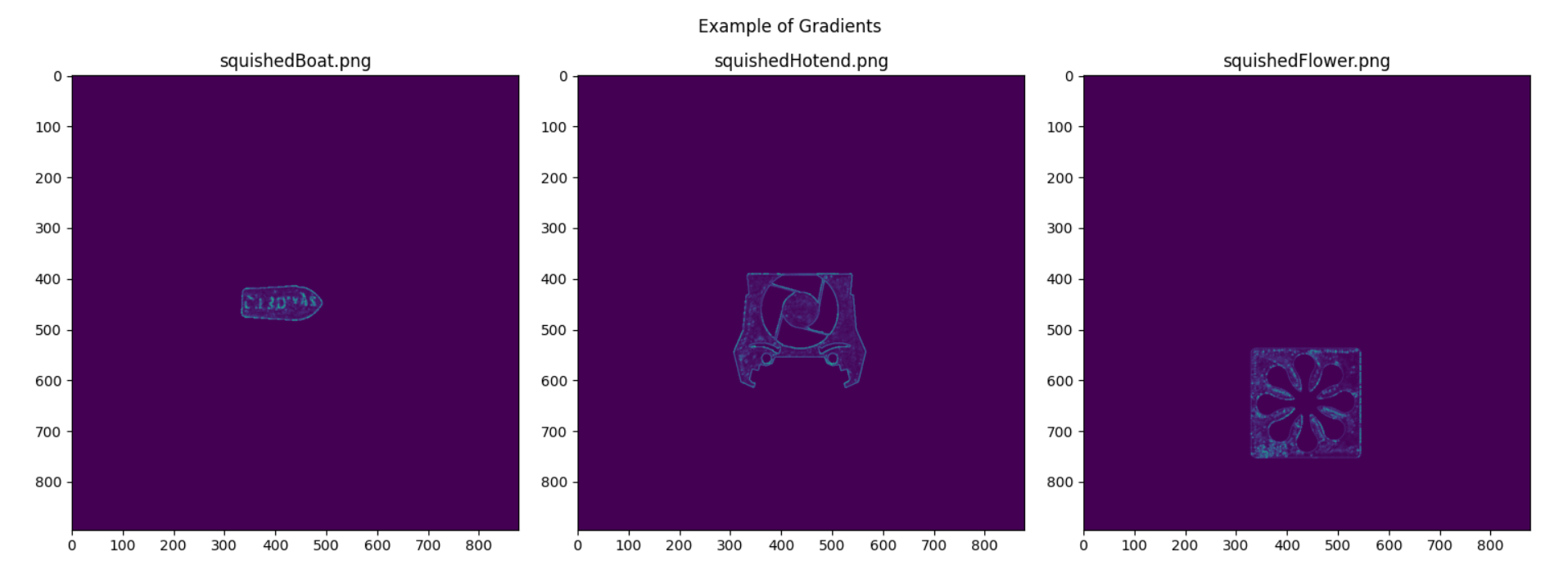
Figure 14: Example gradients of squished layers
Notice that near fine details, there are brighter turquoise highlights, which indicate an increased magnitude in the gradient. In the boat plot, the text has a higher gradient, and in the flower, the model’s designer’s signature is highlighted. These increased gradients made it difficult to determine thresholds that would properly suit the three types of layers. To start determining thresholds, the edge density, mean and variance of the image were calculated on a squished, high, and perfect rectangle.
| File | Edge Density | Mean | Variance |
|---|---|---|---|
| perfectRectangle.png | 0.00223 | 0.50671 | 3.33052 |
| squishedRectangle.png | 0.00318 | 0.61332 | 5.26998 |
| highRectangle.png | 0.02511 | 2.88897 | 51.08978 |
Table 3: Rectangle Gradient Analysis
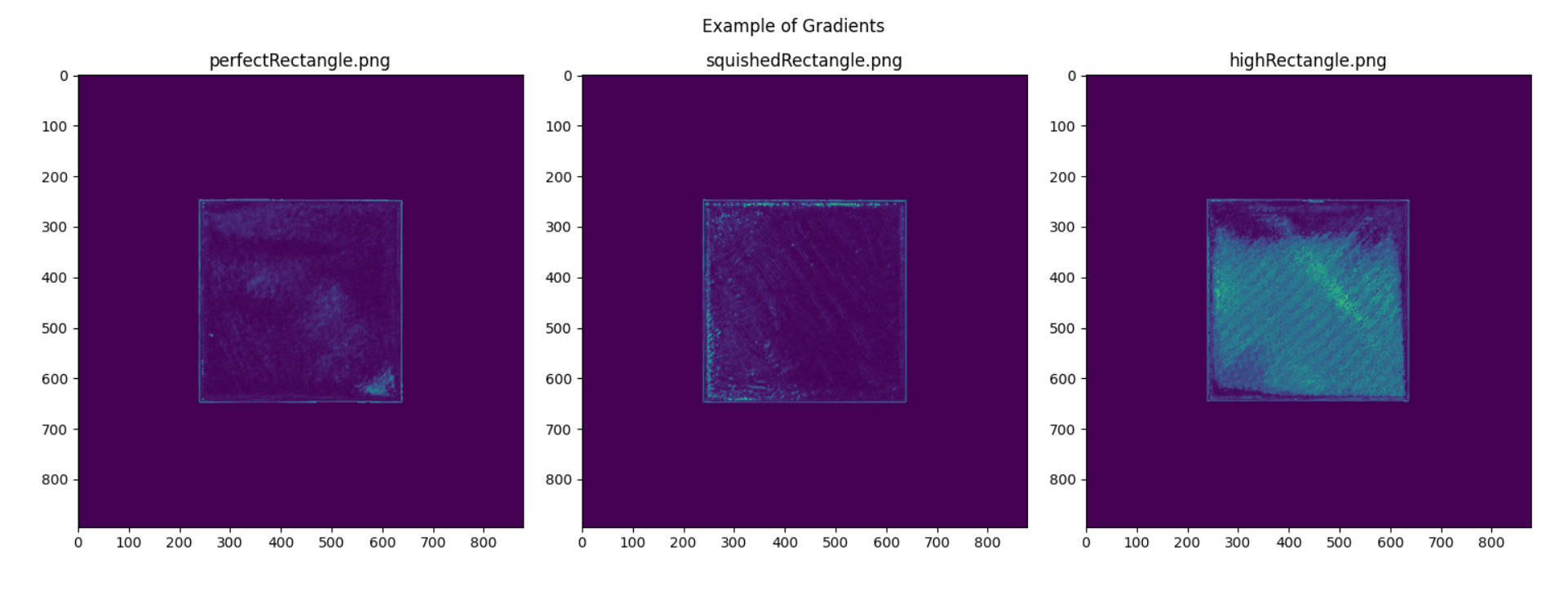
Figure 15: Gradients of a perfect, squished and high rectangles
Based on these initial results, thresholds were set to appropriately identify each classified layer. For a perfect layer, the edge density must be less than 0.0025 with either a mean less than 0.6 or a variance below 3.5. For a squished layer, the edge density must be less than 0.004 and greater than 0.003 or the mean has to be above 0.6 with a variance below 10. Everything else was classified as a high layer. However, when applying these thresholds to another, smaller object, a boat, it was found that it would misidentify the classes.
| File | Edge Density | Mean | Variance | Expected | Output |
|---|---|---|---|---|---|
| perfectBoat.png | 0.0014 | 0.08088 | 1.35596 | Perfect | Perfect |
| squishedBoat.png | 0.00047 | 0.06113 | 0.70453 | Squished | Perfect |
| highBoat.png | 0.00246 | 0.14515 | 3.07877 | High | Perfect |
Table 4: Initial Boat Gradient Analysis
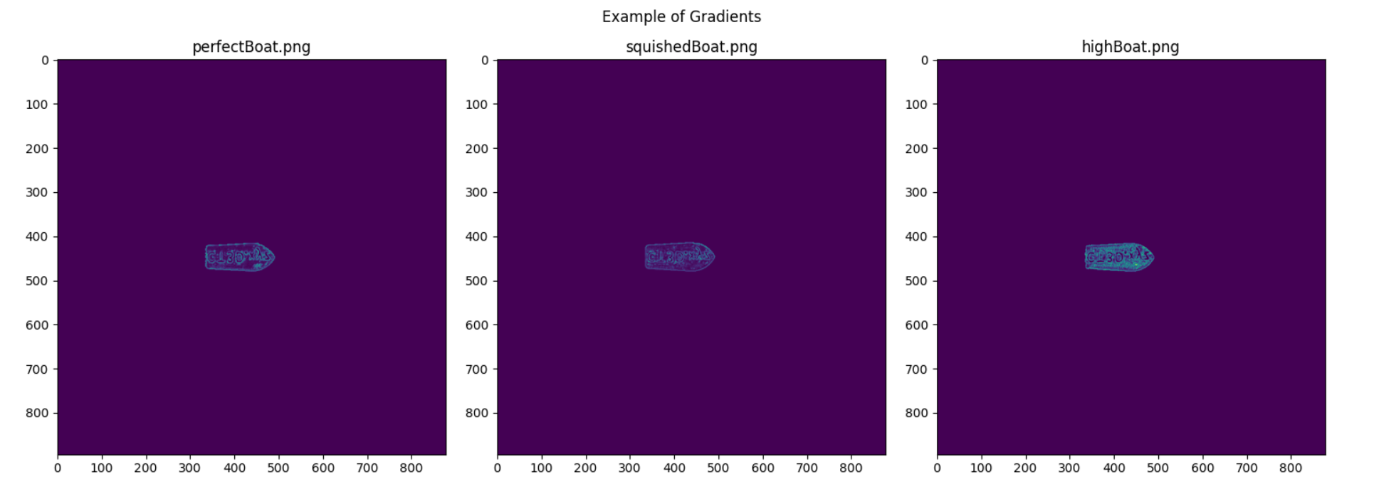
Figure 16: Gradients of a perfect, squished and high boats
Initially, these results were confusing to view, as the statistics did not follow a similar trend to the rectangles. Upon careful inspection of the first layers, the smaller boat had characteristics that aren’t apparent on a flat plot of an object. Due to the text on the boat and the small footprint, the edges are more apparent. Additionally, variance is overall lower when compared to the rectangle examples. This is most likely due to the smaller footprint of the print. Regardless of what is causing these differences, the perfect threshold was amended to be tighter. Making sure the edge density is within 0.001 and 0.0023 stopped everything from being labeled as perfect.
| File | Edge Density | Mean | Variance | Expected | Output |
|---|---|---|---|---|---|
| perfectBoat.png | 0.0014 | 0.08088 | 1.35596 | Perfect | Perfect |
| squishedBoat.png | 0.00047 | 0.06113 | 0.70453 | Squished | Squished |
| highBoat.png | 0.00246 | 0.14515 | 3.07877 | High | High |
Table 5: Final Boat Gradient Analysis
After fine-tuning new thresholds, we then tested on a new set of medium-sized objects.
| File | Edge Density | Mean | Variance | Expected | Output |
|---|---|---|---|---|---|
| perfectHotend.png | 0.00321 | 0.25263 | 3.95123 | Perfect | Squished |
| squishedHotend.png | 0.00261 | 0.19471 | 2.58402 | Squished | Squished |
| highHotend.png | 0.00517 | 0.37255 | 6.67883 | High | High |
Table 6: First Hotend Gradient Analysis
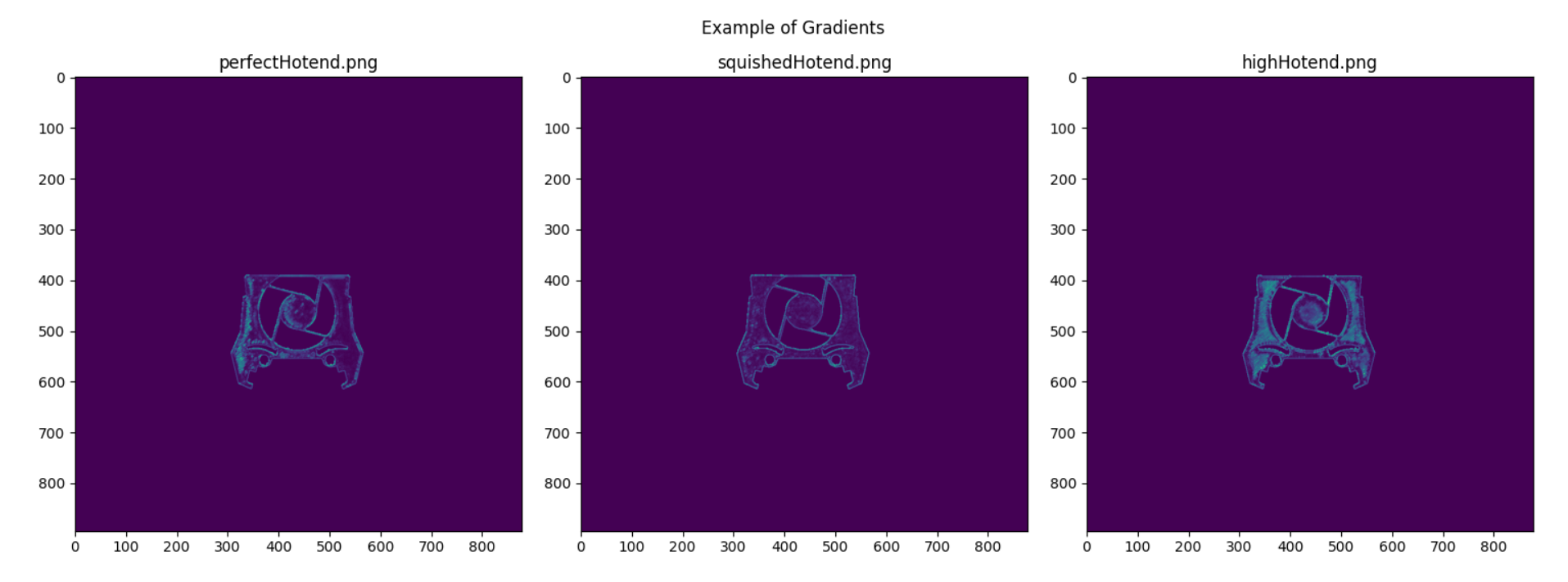
Figure 17: Gradients of a perfect, squished and high on a medium sized object
These thresholds demonstrate two correct outputs, but the perfect threshold is a bit too tight. Increasing the edge density requirement to 0.0035 solves this tight threshold issue.
| File | Edge Density | Mean | Variance | Expected | Output |
|---|---|---|---|---|---|
| perfectHotend.png | 0.00321 | 0.25263 | 3.95123 | Perfect | Perfect |
| squishedHotend.png | 0.00261 | 0.19471 | 2.58402 | Squished | Perfect |
| highHotend.png | 0.00517 | 0.37255 | 6.67883 | High | High |
Table 7: Second Hotend Gradient Analysis
Changing this threshold made the squished hotend output to be incorrect. Adding a minimum to the perfect mean threshold of 0.2 solves this issue.
| File | Edge Density | Mean | Variance | Expected | Output |
|---|---|---|---|---|---|
| perfectHotend.png | 0.00321 | 0.25263 | 3.95123 | Perfect | Perfect |
| squishedHotend.png | 0.00261 | 0.19471 | 2.58402 | Squished | Squished |
| highHotend.png | 0.00517 | 0.37255 | 6.67883 | High | High |
Table 8: Final Hotend Gradient Analysis
These experiments were repeated multiple times until the following thresholds were set:
Perfect: .001 < edge density < .00361 and (0.2247 < mean < 0.6 or 1 < variance < 2)
Squished: edge density < .0009 or (.17 < mean < .62 and 2.4 < variance < 6.4)
High: edge density > 0.0022 and variance > 3 and mean > 0.1
Testing these thresholds on thirty samples, ten of each class provides the following results.
| File | Edge Density | Mean | Variance | Expected | Output |
|---|---|---|---|---|---|
| perfectRectangle.png | 0.00223 | 0.50671 | 3.33052 | Perfect | Perfect |
| perfectVoron.png | 0.00334 | 0.22663 | 3.5213 | Perfect | Perfect |
| perfectBoat.png | 0.0014 | 0.08088 | 1.35596 | Perfect | Perfect |
| perfectHotend.png | 0.00321 | 0.25263 | 3.95123 | Perfect | Perfect |
| perfectTest.png | 0.002 | 0.13293 | 1.88548 | Perfect | Perfect |
| functionalExtruder.png | 0.00214 | 0.27792 | 2.85508 | Perfect | Perfect |
| perfectFox.png | 0.00358 | 0.26784 | 4.38303 | Perfect | Perfect |
| perfectFlower.png | 0.00309 | 0.23597 | 3.54011 | Perfect | Perfect |
| perfectWatch.png | 0.00269 | 0.28397 | 3.48966 | Perfect | Perfect |
| perfectPrusa.png | 0.00227 | 0.29056 | 3.0353 | Perfect | Perfect |
| squishedRectangle.png | 0.00318 | 0.61332 | 5.26998 | Squished | Squished |
| squishedVoron.png | 0.0029 | 0.2236 | 2.83075 | Squished | Squished |
| squishedBoat.png | 0.00047 | 0.06113 | 0.70453 | Squished | Squished |
| squishedHotend.png | 0.00261 | 0.19471 | 2.58402 | Squished | Squished |
| squishedTest.png | 0.00302 | 0.17357 | 2.54252 | Squished | Squished |
| squishedExtruder.png | 0.00374 | 0.43697 | 5.96555 | Squished | Squished |
| squishedFox.png | 0.00435 | 0.33629 | 6.39009 | Squished | Squished |
| squishedFlower.png | 0.00173 | 0.2063 | 2.49509 | Squished | Squished |
| squishedWatch.png | 0.00395 | 0.51772 | 6.26249 | Squished | Squished |
| squishedPrusa.png | 0.00365 | 0.48422 | 4.67597 | Squished | Squished |
| highRectangle.png | 0.02511 | 2.88897 | 51.08978 | High | High |
| highBoat.png | 0.00246 | 0.14515 | 3.07877 | High | High |
| highVoron.png | 0.0063 | 0.45052 | 8.48229 | High | High |
| highHotend.png | 0.00517 | 0.37255 | 6.65883 | High | High |
| highTest.png | 0.00335 | 0.22468 | 4.07882 | High | Squished |
| highExtruder.png | 0.00428 | 0.42682 | 6.56383 | High | High |
| highFox.png | 0.00652 | 0.45275 | 10.15104 | High | High |
| highFlower.png | 0.0049 | 0.36666 | 6.1754 | High | Squished |
| highWatch.png | 0.00697 | 0.85351 | 13.89035 | High | High |
| highPrusa.png | 0.00932 | 0.65029 | 9.75917 | High | High |
Table 9: Gradient Analysis of First-Layer Photos
Out of 30 results, 28 provided correct predictions for an accuracy of 93%. Additionally, these inappropriate predictions were labeled as squished compared to high. This is less of an issue as the goal of the system is to pause the print when the first layer is not perfect, which with this output would still appropriately pause the printer. Additionally, the squished thresholds could be altered further to make it so it doesn’t misclassify high layers.
For the spaghetti detection, we needed to transform the basic YOLOv11 model into a model that specifically looks for the 3D printer filament to become spaghetti-shaped. While this may be a hefty process, the Python library that enables the usage of YOLOv11, ultralytics, makes this process very easy with simple functions for all steps of tuning the model [5]. Next, we also need lots of labeled data, in this case, filament spaghetti images, so that the machine learning model has enough context to correctly understand what this failure looks like to then identify it in new situations. Earlier, we mentioned an open-source dataset on roboflow named “Spaghetti 3D Dataset” exists, and this is the source of all our datasets [3]. This dataset contains three sets of images: a training set, a validation set, and a test set, all of which have corresponding labels. Each of these types of sets plays a crucial role in the training of any machine learning algorithm.
First, we train the model by feeding the entire training set into the model as an input and see how it detects filament spaghetti, comparing that output to the training set labels, and then adjusting the model’s weights so it better understands what is important to look for in the images. After one whole pass of the training set, called an epoch, we test the adjusted model on the validation set to record how well it performs. The validation and test sets contain images outside the training set, so we refer to these sets as unseen data. After repeating this process for all epochs, we can test the accuracy of our model by running inference on the test set. This particular test set only contains images where filament spaghetti is present, so by checking how many times the model detects spaghetti in the image and dividing that value by the number of items in the test set, we calculate the accuracy of the model. This works because we want to have a detection algorithm that only needs to recognize when spaghetti is in the scene. While the location of the spaghetti is important, it is not crucial for our needs. We then test the model’s ability to not return false positives, so we run a separate test on the set of images we used during the gradient analysis. Below, we specify the training hyperparameters and the test performances.
| Hyperparameters | Meaning | Value |
|---|---|---|
| epochs | # of passes through training data | 75 |
| imgsz | Image size (N x N) | 640 |
| optimizer | Weight adjustment algorithm | ‘auto’ |
| batch | Batch size | -1 (GPU optimized) |
| lr0 | Initial learning rate | 5e-3 |
| lrf | Final learning rate as ratio of lr0 | 1e-2 |
| weight_decay | Prevents bias from large weights | 5e-4 |
| single_cls | Treats multi-class datasets as single-class | True |
| warmup_epochs | # of epochs to increase learning rate | 3 |
| deterministic | Sets training as deterministic or random | False |
| device | Specify CPU(s) or GPU(s) | 0 (one/first GPU) |
Table 10: Hyperparameters used during YOLOv11 training via ultralytics model.train()
The training set contained 515 labeled images. Both the validation and testing sets contain 100 labeled images. For the hyperparameters, there are two that need more clarification. Firstly, we set single_cls to because the datasets contained two classes, “spaghetti” and “stringing”, however, our model should detect these all the same so we bunch both classes together into a single class [6]. Secondly, we set deterministic to false to introduce some randomness that allows the model to possibly outperform the deterministic model, as well as improve training speed [6].
| Testing Dataset | Contains | Model Accuracy |
|---|---|---|
| Spaghetti Dataset Test Set | Filament Spaghetti Images | 95/100 → 95% |
| First Layer Prints | Non-Spaghetti Images | 25/31 → 80.65% |
| - | - | Overall: 120/131 → 91.6% |
Table 11: Accuracy of trained YOLOv11 Model
By testing the trained YOLO model on images of both spaghetti and non-spaghetti images, we got mostly accurate results. In fact, across both datasets, the accuracy was 91.6%, which is fantastic given the datasets used. For the most part, open-source and labeled datasets of quality filament spaghetti spaghetti are far and few, with the “Spaghetti 3D Computer Vision Project” dataset being the most available. This dataset is filled with images that have been collected from the internet and then manually labeled, so there is no consistency in the angle of the camera or the quality of the photos. From our camera angle, much of the printing bed is exposed, which was not common in the dataset training photos, leading to a few mislabelled images of the first layer prints. Furthermore, it appears that some patterns on the prints themselves can be recognized as spaghetti, namely the flower pattern. This may be a residual bias from the training data. All things considered, the performance of the YOLO model is exceptional. Future work that can be done to prevent mislabelling could be a second gradient analysis of the box where spaghetti is located to confirm or deny the presence of spaghetti.
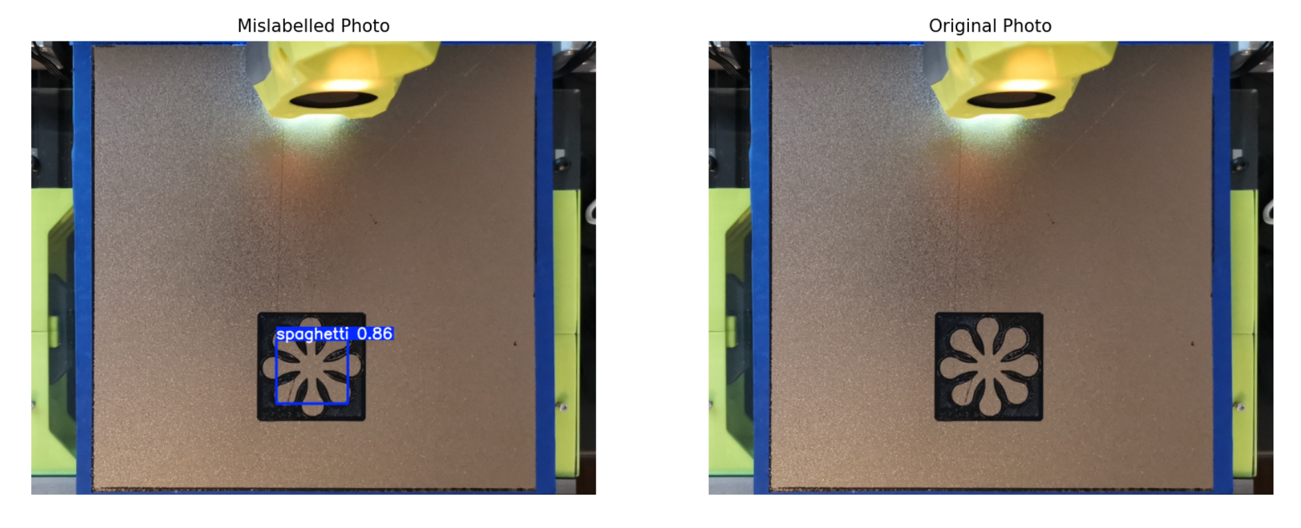
Figure 18: Mislabeled Flower image. Flower photos were 4 of 6 mislabeled photos
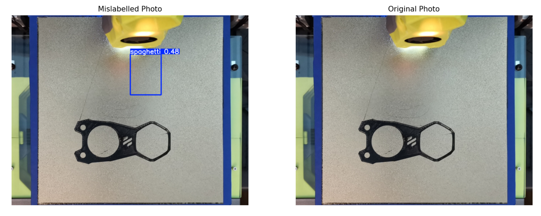
Figure 19: Mislabeled Voron image. Invisible detections made up the last 2 mislabeled images
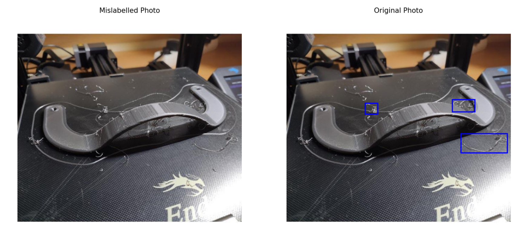
Figure 20a: Unlabeled spaghetti image. Strands like this may not have beem represented in the testing dataset
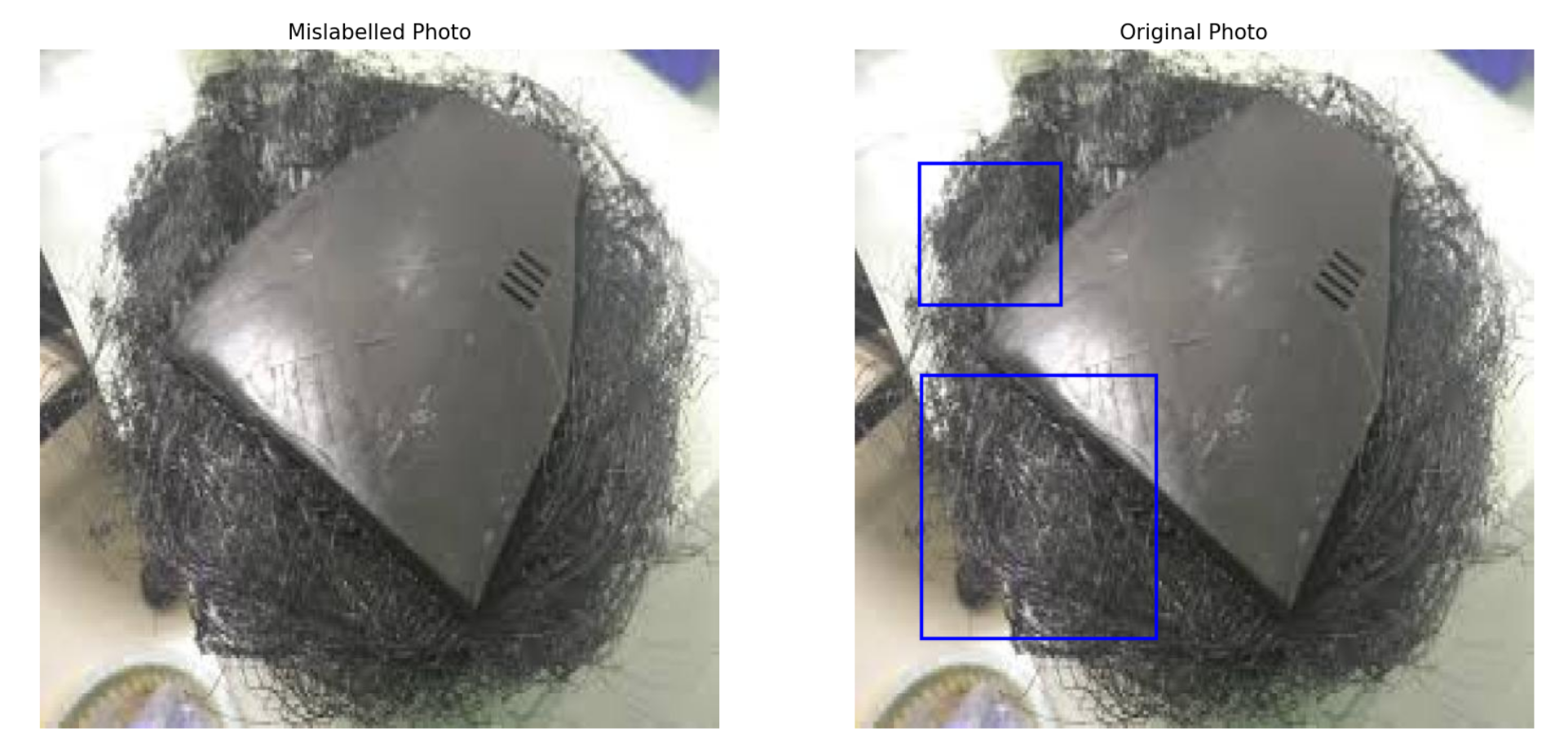
Figure 20b: Unlabeled spaghetti image. Excessive spaghetti was not recognized. Ideally the YOLO detects spaghetti before it gets to this point
We can compare this to a naive approach, which is the default YOLOv11 model. With the same methods as above, we can test on both the test set and our print bed pictures, checking if it makes a classification.
| Testing Dataset | Contains | Model Accuracy |
|---|---|---|
| Spaghetti Dataset Test Set | Filament Spaghetti Images | 44/100 → 44% |
| First Layer Prints | Non-Spaghetti Images | 24/31 → 77.42% |
| - | - | Overall: 68/131 → 51.9% |
Table 12: Accuracy of untrained YOLOv11 Model. The naive model is unsuitable for our project's use case
Note 1: The tests for the spaghetti test set checked if anything was classified by the model. All of these classifications were not identified as “spaghetti”, so the real accuracy would be 0% for the incorrect classification in the first dataset.
Note 2: In the tests for the non-spaghetti images, the correct classification is none at all. These are times when the default model does not recognize anything in the image
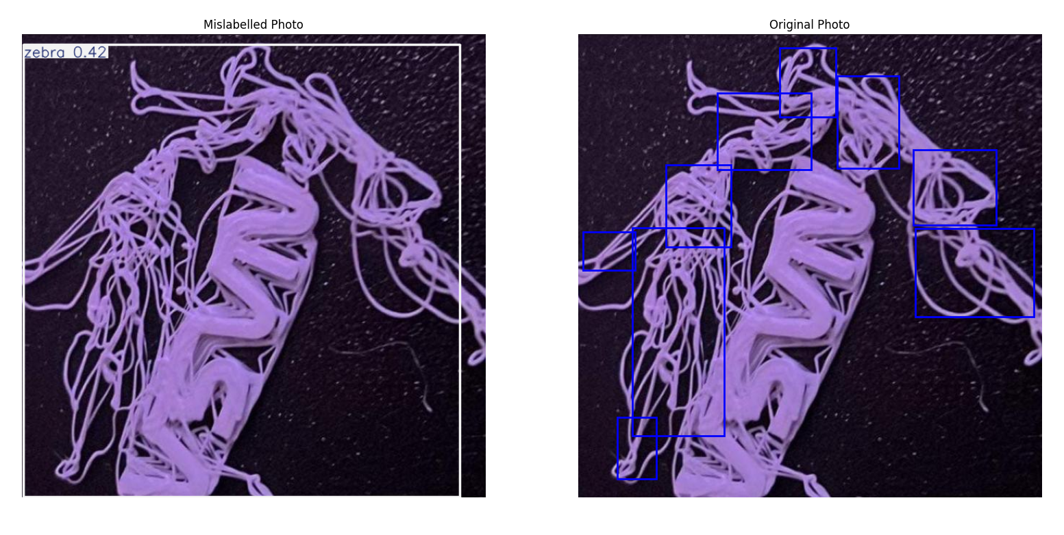
Figure 20c: Mislabeled spaghetti image. Untrained model believes the image shows a zebra
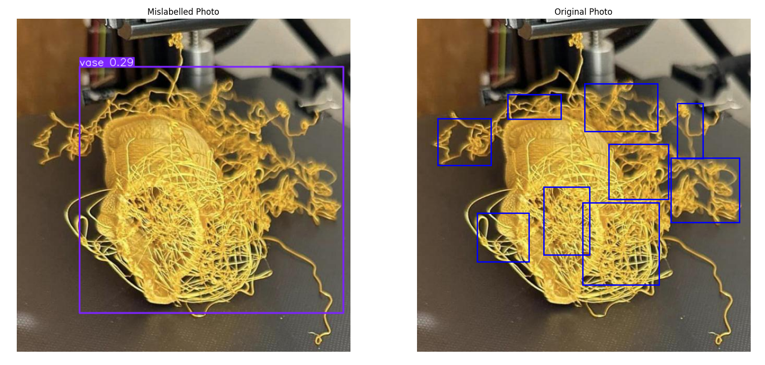
Figure 20d: Mislabeled spaghetti image. Untrained model believes the image shows a vase
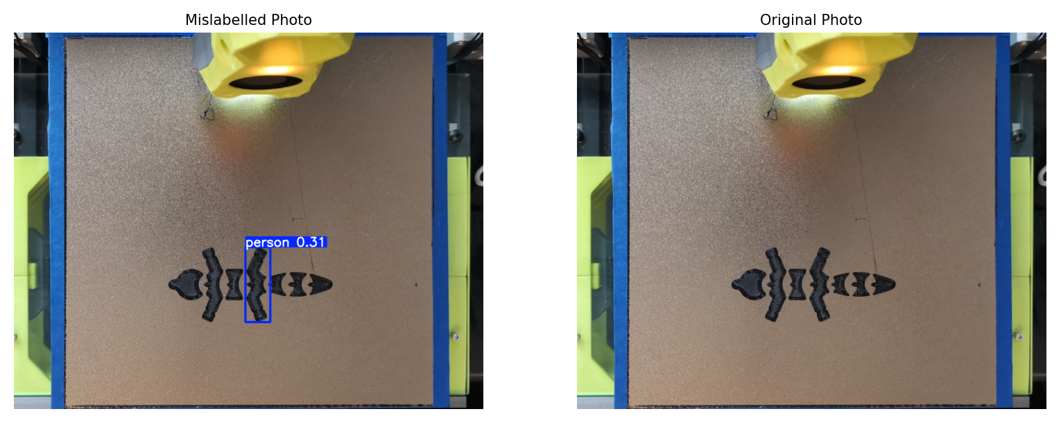
Figure 20e: Mislabeled spaghetti image. Untrained model believes the image shows a person
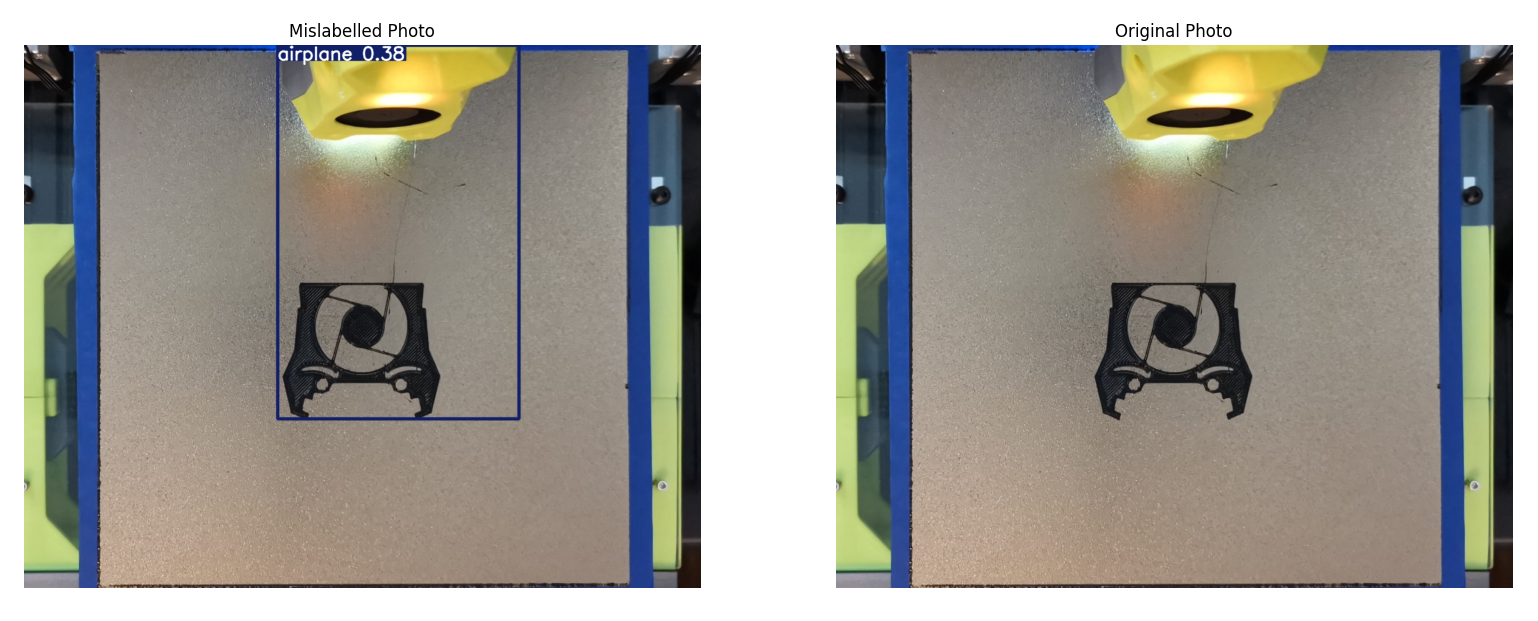
Figure 20f: Mislabeled spaghetti image. Untrained model believes the image shows an airplane
Qualitative Results
Figure 21: watch.png before skew correction
Figure 22: watch.png after skew correction
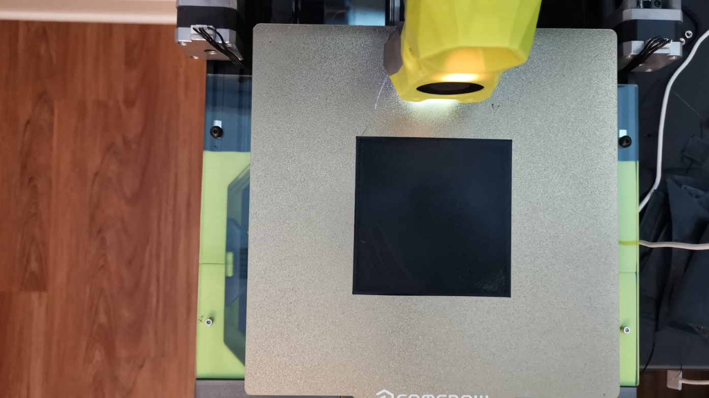
Figure 23: rectangle.png before skew correction
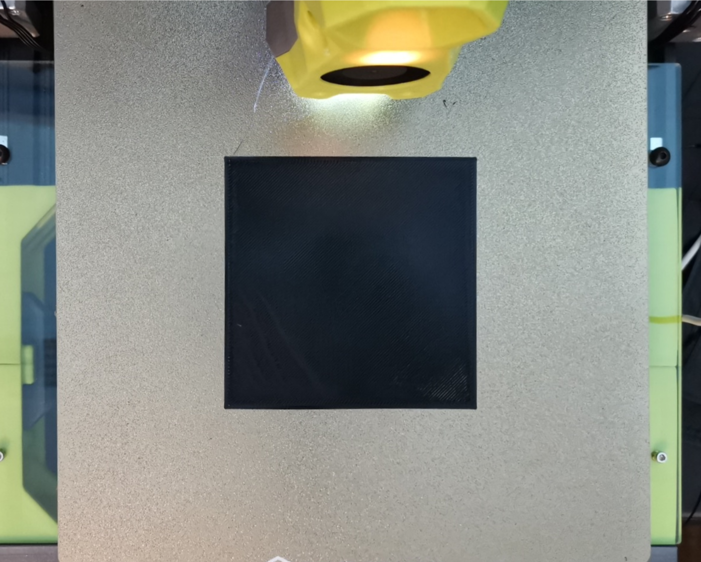
Figure 24: rectangle.png after skew correction
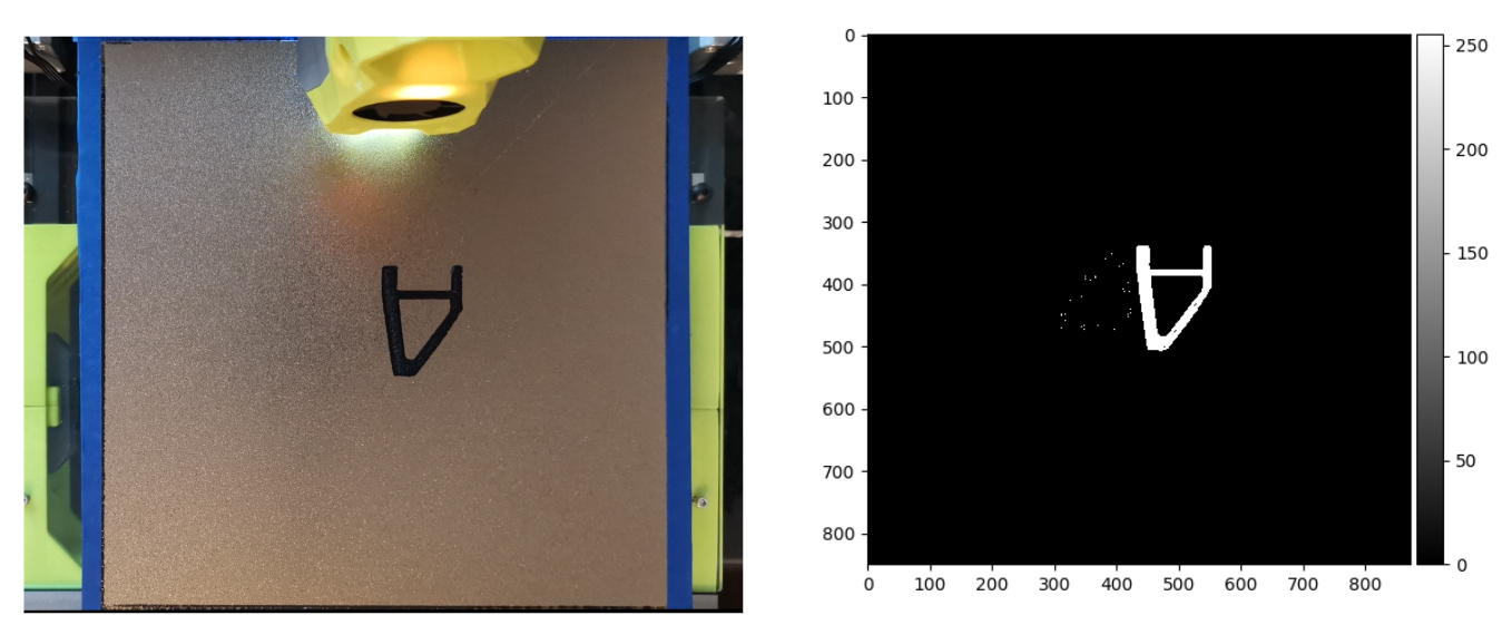
Figure 25: Missing object detection - Correctly predicted
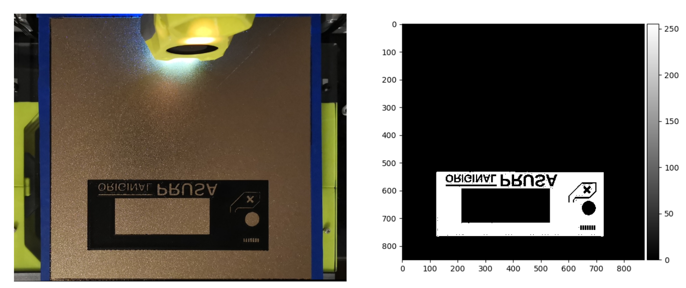
Figure 26: Missing object detection - Correctly predicted
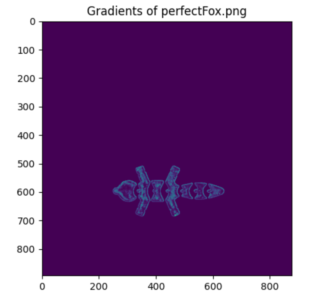
Figure 27: Gradient of a Fox - Deemed perfect - Correct prediction
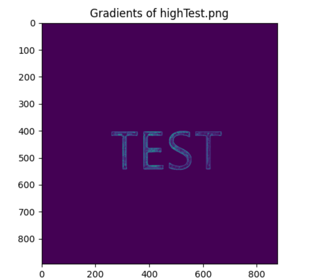
Figure 28: This is due to the inconsistencies of the mean and variance of the gradients. Having it raised and squished in various locations brought inconsistencies.
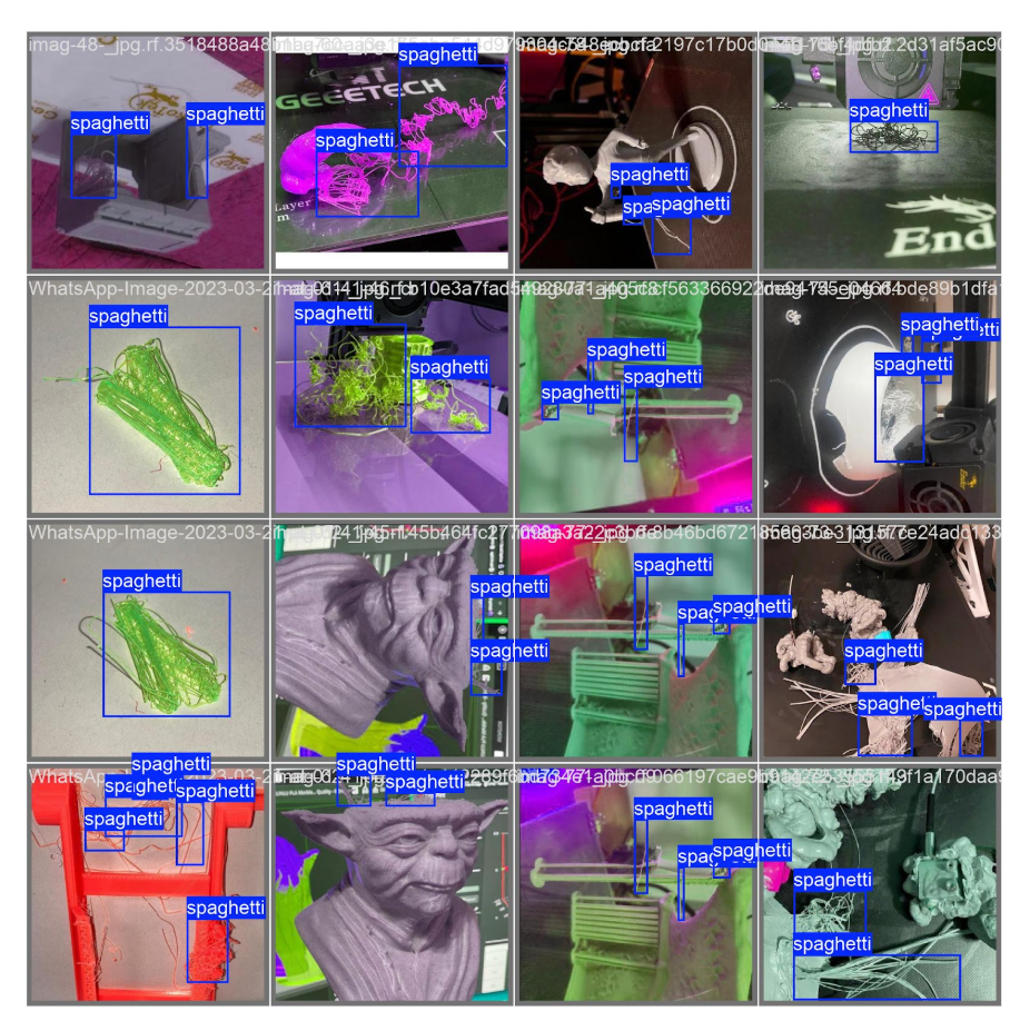
Figure 29: Actual Spaghetti Locations from Validation Set
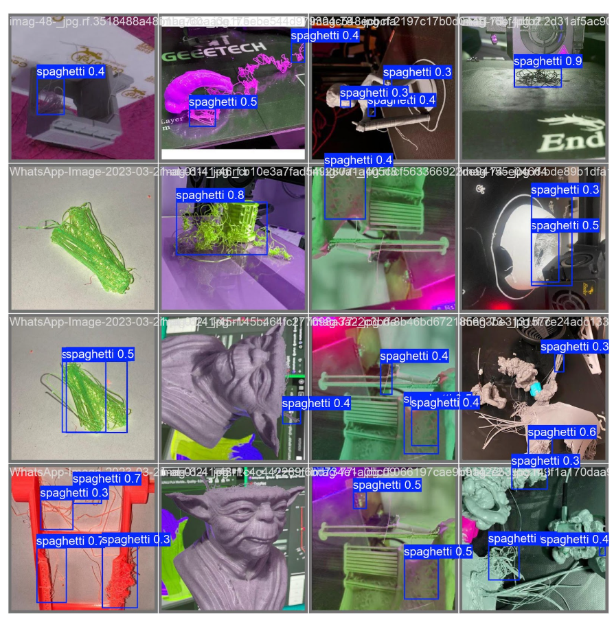
Figure 30: Predicted Spaghetti Locations on Validation Set
Conclusion
By integrating methods from computer vision, digital image processing, and machine learning, we presented a system that will analyze the quality of the first layer of 3D printed objects, reducing the number of failed prints while optimizing time and cost efficiency by detecting defects. This system has multiple preventative measures, the first being our trained YOLOv11 model that can detect if the filament begins to “spaghetti” in real time with an accuracy of ~92% from the camera mounted on the 3D printer. After the first layer is successfully printed, a photo is taken, and we align this photo to a simulated first-layer image by performing a 2D homography transformation with over 99% accuracy. Next, our second preventative measure takes place, an object detection algorithm that utilizes global thresholds to binarize our bed plate photo to find the difference between the real-world and simulated images and find the percent error. If the error is too high or 0%, we know at least one object is missing from the print bed. Finally, the third preventative measure takes place and performs a quality check of the print objects themselves by using a gradient analysis which correctly determines if the z-offset of the print was too high, too low, or just right 93% of the time.For later developments, we would like to introduce a few things to potentially make this system more stable. Firstly, by increasing the spaghetti dataset size, the YOLO model would recognize more diverse scenarios of spaghetti, and may also remove the false positives from the flower-shaped objects. This could be supplemented with labeled images from our camera setup, preventing false positives on the surface of the print bed while getting a more personalized batch of data specific to angle, lighting, and filament. We also briefly mentioned using a second gradient analysis step on the image within the boxes of the YOLO detection to further prevent false positives. Secondly, parts of the 3D printer setup could also be improved, such as getting a non-reflective print bed, increasing the light brightness for more consistency, and adjusting the camera to better represent the simulated view of the first layer. Lastly, swapping to other coding languages such as MATLAB or C++ may have quicker computational times, increasing the speed of inference for each of our detection algorithms.
Overall, we are satisfied with the project we have created and are excited to share this with you. By improving the quality of 3D printed first layers, we are setting the foundation for higher quality additive manufacturing capabilities and saving precious time and materials.
References
[1] https://moonraker.readthedocs.io/en/latest/web_api/[2] https://kili-technology.com/data-labeling/machine-learning/yolo-algorithm-real-time-object-detect
[3] https://github.com/ultralytics/ultralytics
[4] https://universe.roboflow.com/3d-printing-failure/spaghetti-3d
[5] https://scikit-image.org/docs/stable/api/skimage.metrics.html#skimage.metrics.structural_similarity
[6] https://docs.ultralytics.com/modes/
[7] https://docs.ultralytics.com/modes/train/#train-settings